What happens when peak running time is wrong
A running time that works later in the day might fall apart during peak at 8am. When peak journeys aren't given enough time, buses run late and eat into their recovery time. If the delay is longer than the recovery time, it carries into the next trip. Give them too much time, and buses might run early – and passengers who arrive on time miss the bus completely.
The fallout of an unfit timetable affects almost everyone involved in running the network:
- Schedulers and planners need evidence to justify a retime. Without a clear view of when running time drifts, a change takes longer to build and is harder to defend to an authority, a board, or unions.
- Operations and performance managers see persistent peak lateness and chase drivers or control decisions, when the real cause is a timetable that doesn’t allow journeys enough time.
- Drivers are pushed to make up time they weren’t given, with less recovery time between trips.
- Operators working to contracted punctuality targets can miss their KPIs and, where contracts apply them, face financial penalties for late running that started with the timetable.
- Authorities need independent evidence to approve or challenge an operator's proposed timetable changes, and to report peak punctuality to senior management.
- Bid and tender teams rely on realistic peak running times to work out how many vehicles and drivers a route they’re bidding on needs. Underestimate these numbers and you risk missing contractual targets once you win; overestimate them and your bid costs more than it needs to.
In every case, the same evidence is needed: exactly when in the day actual running times drift from schedule, and by how much.
Until now, building that view meant repeatedly exporting running times and rebuilding an hourly-based view in Excel or Power BI. With schedulers and planners doing this by hand for every route they reviewed, the manual effort mounted up fast.
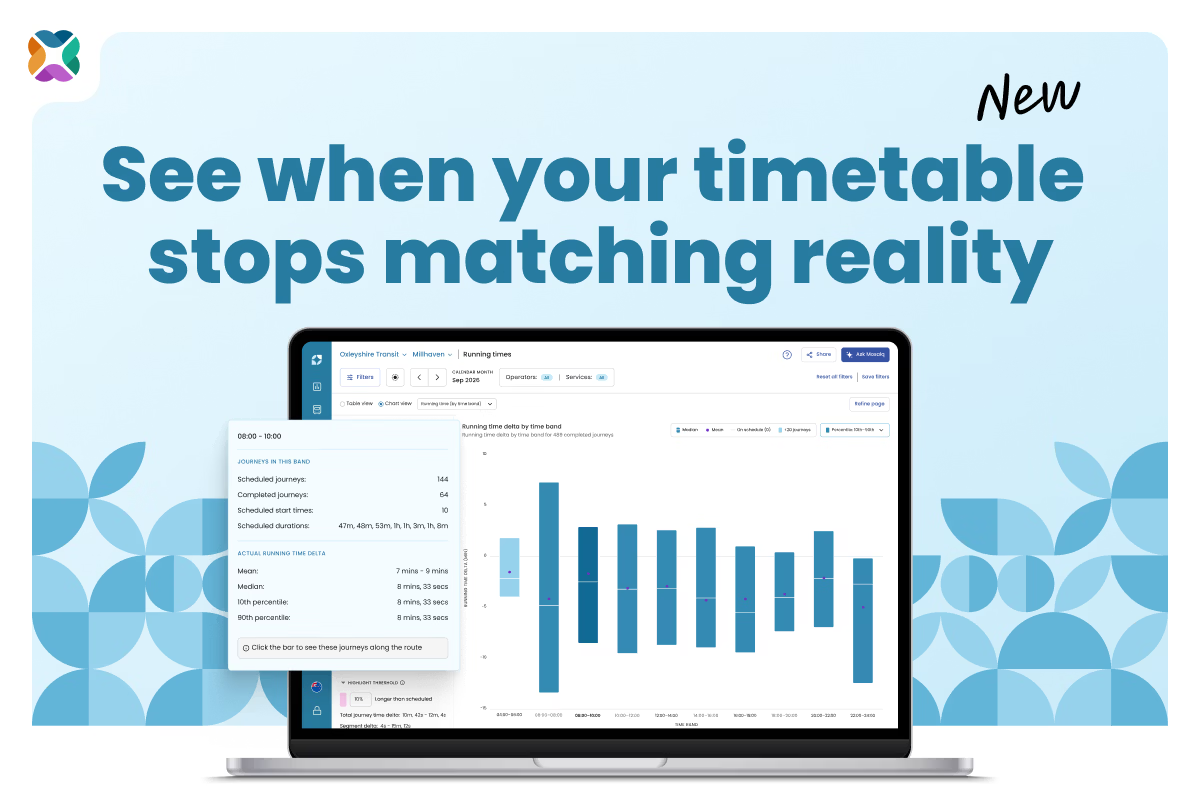
Mosaiq Insights by Snapper Services now does that work for you. The new Running time (by time band) chart shows how far journeys run over or under schedule across the whole service day, so you can quickly spot the time bands that need attention, find out exactly where on the route time is lost, and export the evidence for your running time analysis report.
See running times across the whole service day
The Chart view on the Running times page now has a Select chart dropdown with two charts:
- Running time (along journey): the chart you already know, showing running time segment by segment
- Running time (by time band): the new chart, showing how far journeys ran over or under schedule at different times of day
The new chart splits the service day into fixed two-hour time bands, counted from 00:00. Each journey sits in the band its scheduled start time falls in. Journeys that start after midnight stay with the service day they belong to, so a band such as 00:00–02:00 (+1) appears at the end of the axis for some variants.
Each bar shows the running time delta for the journeys in that band: actual running time minus scheduled running time. Zero means on schedule. The bar spans a percentile range (10th to 90th percentile by default, covering the middle 80% of journeys), with a tick for the median and a dot for the mean. You can switch to the 20th/80th or 25th/75th percentile to remove more outliers.
Showing the range, median, and mean together is deliberate. Some transport teams measure running times using averages; others use percentiles. The chart gives you both, so you can work with the number you already report on.
How to read the Running times by time band chart
| What you see |
What it means |
| A short bar sitting across the zero line |
The timetable matches reality, and journeys are consistent |
| A bar wholly above zero |
Journeys in this band consistently take longer than scheduled |
| A bar wholly below zero |
Journeys in this band consistently run quicker than scheduled |
| A tall bar |
Running times vary widely in this band |
| A mean well away from the median |
A few outlier journeys are skewing the average |
| A lighter shaded bar |
Fewer than 20 completed journeys, so treat the result with caution |
| A tooltip but no bar |
Journeys were scheduled in this band, but none were completed |
Building the case for a peak retime: a worked example
This example follows a scheduler preparing a running time analysis report before a timetable change.
The scenario: a newly created express route that carries commuters into a city centre during the morning peak. Customer feedback and driver reports say the morning journeys are tight, and the scheduler wants evidence before adding running time. The analysis covers one quarter of data.
Start with the big picture
Across the quarter, the route is falling short:
- It's 4.7% below its punctuality KPI target.
- 14.3% of journeys are late at the last stop.
- 12.6% of journeys run longer than scheduled.
The inbound variant is the main cause. 19% of its journeys run longer than scheduled, and it's 3.2% below its punctuality KPI target. Its data quality is strong enough to act on: 98.1% of its 520 scheduled journeys were matched, and 60% of those were completed.
Spot the bands that drift
The Running time (by time band) chart for the inbound variant shows two different problems in the morning:
- 08:00–10:00 needs more time. The bar sits above zero, with a median overrun of 3m 56s, and the slowest 10% of journeys run more than 7m 42s over schedule. With 115 completed journeys in the band, the sample is large enough to trust – making this the retime candidate.
- 06:00–08:00 is unpredictable. The median overrun is a smaller 1m 38s, but the bar is much taller, indicating increased variation. That points to a predictability problem rather than a running time problem, so adding time won't fix it.
Check whether every weekday behaves the same
Weekdays don't always behave alike, so it's worth checking before applying the same fix to all of them. To check how a time band performs on different days, change the Days of the week filter in the Refine page modal, then compare the peak bands. In this example, the 08:00–10:00 overrun appears consistently across the week, so a single weekday retime is justified.
Find the exact stretch of route losing time
Select the 08:00–10:00 band. The Running time (along journey) chart opens, filtered to only the journeys that start in that window, and the band appears as a Time band filter chip beside Refine page.
Here, most of the overrun builds up on the stretch of route through the city centre, where commuter buses queue in peak traffic. That gives the scheduler a specific, defensible change: add running time to those segments for journeys starting between 08:00 and 10:00.
To take the evidence into your report, use Export while the time band chart is showing. You'll get a CSV with one row per band.
From a hunch about the peak to evidence you can defend
The Running time (by time band) chart is available now to all Mosaiq Insights users, including those on the Free plan, and there's nothing to set up. Next time you open Running times, choose it from the Select chart dropdown and see when in the day your timetable stops matching reality.
Stay connected
Want to be the first to know about the latest Mosaiq updates? Make sure to check our Release Notes regularly. To get monthly updates direct to your inbox, sign up to our mailing list.